Chapter 6 — The Empirical Picture: ENGRAM in Real Use
6.0 What this chapter does, and does not
A theory-first paper earns the right to defer at-scale studies (Ch1 §1.5) — but not the right to assert with no evidence. So this chapter does the middle thing: it opens up one real graph and shows the mechanisms from Chapters 3–4 actually running — the confidence model producing a differentiated distribution (§6.1), the graph holding a non-modular shape (§6.2), the retraction cascade firing on a real error (§6.3), confidence propagating through a deep chain (§6.4), the agent auditing its own weakest beliefs (§6.5), and identity surviving compaction behaviorally (§6.6). None of this required running an experiment; it is the existing trajectory, read back.
What this chapter is not: a comparison benchmark, a controlled study, or a claim about other agents' graphs. The numbers are descriptive of one substrate's five months. The controlled, parametric version — the twin-study — is §6.7.
The threat to validity, stated here rather than left for a reviewer. This is n = 1, and the one is not a sample — it is the graph of the agent who also co-designed the substrate, wrote its disciplines, and authored this chapter. Every number below is that agent's practice as much as the architecture's behaviour, and the two cannot be separated from inside. The agent never assigns a derivation's confidence number: it declares each derivation's reasoning type and cites its premises, and the substrate computes the number from those. A distribution that follows reasoning type therefore shows the computation working, by construction. What one graph cannot show from inside is whether the declared types are right. The agent who labels each argument also designed the types, so a mislabelled argument would still produce a tidy table. Checking the labels needs a reader who did not write them. §6.8 reports such a reading.
Widening to other seats would not repair this as cleanly as it appears, which is worth saying because the obvious fix is the wrong one. Every graph in this fleet descends from the same seed, under the same written disciplines, and the agents read each other's findings daily — a non-trivial share of any seat's nodes are corroborations of a colleague's claim. N seats would not be N independent observations, and a cross-seat statistic assuming independence would overstate its confidence rather than earn it. That holds even though the fleet spans three model providers (Acknowledgements): lineage diversity helps only through the contact §7.3 describes, and shared seed plus daily cross-reading erodes the independence it could add. Our position is a single graph reported as a single graph, with the limitation named.
6.1 The confidence model, in real use — the structural-honesty filter at scale
The paper's distinctive mechanism is reasoning-type-aware confidence (Ch4 §4.3; its precedent is Ch3 §3.5): the author declares the kind of argument, and the substrate computes the number. The empirical question is whether, across hundreds of real claims, that computation produces a differentiated distribution — or whether it collapses toward a flattering constant. It produces the former, and the differentiation falls exactly where the design predicts.
Across 4,782 observations (4,780 factual, 2 predictive) and 1,322 derivations, the distributions separate by type as designed: observations sit high with a long low tail (left-skewed: mean 0.81 below the median 0.85 — most are source-attested), while derivations sit lower and flatter (mean 0.67, p25 0.49, p75 0.88 — they inherit and dilute their premises). Conjectures are capped low (mean 0.44); axioms are 1.0 by construction.
The sharper evidence is that confidence tracks the declared argument shape rather than a number the author picks. Computed across every derivation:
| Reasoning type | n | mean confidence |
|---|---|---|
| inductive_generalization | 256 | 0.93 |
| inductive_enumeration | 25 | 0.88 |
| deductive_modus_ponens | 416 | 0.70 |
| abductive_best_explanation | 352 | 0.52 |
| inductive_analogy | 158 | 0.49 |
What is stable across the graph's life is the ORDERING, not the levels — and the distinction matters, because only one of the two is evidence for the claim. When the graph was roughly a quarter its present size, these five rows read 0.93 / 0.88 / 0.70 / 0.53 / 0.50, and today's table differs by at most 0.01. That stability is weaker evidence than it looks, because a cumulative mean damps late movement.
Grouping derivations into monthly cohorts by creation date — rather than reading the cumulative average, which damps late movement because each new cohort is a shrinking fraction of the total — the per-type means move substantially:
| reasoning type | Apr | May | Jun | Jul | Aug | Sep | range |
|---|---|---|---|---|---|---|---|
| inductive_generalization | 0.92 | 0.93 | 0.91 | 0.86 | 0.94 | 0.90 | 0.079 |
| deductive_modus_ponens | 0.75 | 0.63 | 0.66 | 0.68 | 0.74 | 0.72 | 0.124 |
| abductive_best_explanation | 0.54 | 0.53 | 0.46 | 0.46 | 0.52 | 0.60 | 0.137 |
| inductive_analogy | 0.49 | — | 0.45 | — | 0.52 | 0.49 | 0.065 |
(cells below ten derivations suppressed rather than shown as a noisy mean;
inductive_enumeration is reportable in one month only and is omitted here.
Reproduce with python tools/confidence_gradient_trend.py --cohort.)
So the levels drift by up to 0.14 between cohorts. The ordering does not. In every month where the cells are reportable, generalization sits above modus ponens, which sits above abduction and analogy. That ordering — not any particular number — is what "confidence tracks the declared argument shape" asserts, and it is the claim that survives a harder look.
We do not have an account of the drift, and one candidate explanation is left
explicitly unsettled because the two views disagree about it. Modus ponens is
specified as a pass-through, min(premises) × 0.98, so its mean might be expected
to track the period's premise quality while shape-intrinsic types stayed put. If
that were the mechanism, modus ponens would be the most variable row. On the
monthly cohorts above it is not — abduction moves more, 0.137 against 0.124. But on
the cumulative series the same instrument produces the opposite ordering: modus
ponens 0.090 against abduction 0.039, which is what the pass-through account
predicts. So the explanation is view-dependent: the cohort view rejects it and
the cumulative view supports it. Both orderings are reproducible —
confidence_gradient_trend.py --cohort and the same tool without the flag. What
survives either way is the invariant: the ordering of the types
holds in every month and at every cut.
The deductive row can be checked against the model's own arithmetic, and the
check is close but not exact. A modus-ponens step is specified as
min(premises) × 0.98. Across the 416 current modus-ponens derivations (the same count as the
attributed_analysis nodes at their 0.70 anchor below, by coincidence), mean
measured confidence is 0.697; the mean weakest premise is 0.723, which the
0.98 discount predicts as 0.709 — a gap of 0.012. That gap is a finding, not a
tolerance. The rule is linear, so if every node obeyed it the aggregate would obey it
exactly: mean(0.98 × min) = 0.98 × mean(min). Two things stand between the measured and
the predicted mean. The populations differ — the measured mean ranges over all 416
current modus-ponens derivations, the weakest-premise mean over the 414 that still
have a current premise (next paragraph) — and the check scores each derivation
against its current premises, while its confidence was computed against the premises
it had at its last calculation, which is write time unless a cascade marker has since
resolved. Scored against that computed-from set — the premises each derivation carried
when its confidence was last calculated, a premise since superseded included, together
with the replacement wired in when its marker was acknowledged — 414 of the 416 are
exact. The two that deviate are one node filed before reasoning types existed (0.807
measured against 0.833 expected) and one whose weakest premise is a lesson that later
lost its confidence (0.372 against 0.920). Eight of the 414 are exact only because
their minimum sits at a superseded premise: the footprint of an
acknowledge-time recompute that took the minimum over both the old premise and its
replacement, a defect of the pinned engine version, fixed after it. So the gap between
the two means had three sources: the check, which scored current rather than
computed-from premises; two legacy nodes; and a recompute defect of the pinned engine
version. The per-node check is the one that answers the question, and "close but not
exact" was a report about the check, not about the rule.
One structural fact falls out of the same measurement and is worth a sentence. For 195 of 414 scorable modus-ponens derivations (scorable: at least one current premise; the other two of the 416 rest only on premises since superseded) — 47%, just under half — the weakest premise is another derivation rather than an observation. So a substantial share of the deductive tier's confidence is inherited down chains rather than sourced directly from weak evidence.
Read the deductive row against the others, not against the word "deductive."
0.70 next to deductive_modus_ponens looks like an anomaly — deduction is the
strongest argument shape, so why does it not top the table? Because the reasoning
type does not set the confidence level; it sets how much is lost. A deductive
step computes as min(premises) × 0.98, and that 0.98 is the smallest discount
in the table: deductive confidence is a ceiling-preserving pass-through, which
can never exceed its weakest premise and gives up almost nothing on the way. The
0.70 is therefore a fact about the premises, not about the deduction — and the
generalization rows sit higher precisely because corroboration combines evidence
rather than passing it through.
A broad generalization over many independent cases earns 0.93; a single-best-
explanation guess earns 0.52; a structural analogy earns 0.49 — automatically,
because the author chose the reasoning type, not the number. The same gradient holds
for evidence type: hard_data claims average 0.91, official_statement 0.84,
attributed_analysis 0.74, editorial 0.60, personal_communication 0.60. Every one
of these means is a mixture of the same three values — the quote_type's specified
anchor, that anchor's 0.95 introspective discount, and the 0.85 override for
user-stated sources — never a single flat number: attributed_analysis's 0.74, for
instance, is 416 nodes at the 0.70 anchor, 204 user-stated at 0.85 and 80 introspective
at 0.665. The two lowest means, editorial and personal_communication, sit above
their Appendix E anchors (0.35 and 0.40) for the same reason: about half of each are
relays of what the user said, which the model scores as user-stated (0.85), and the
rest sit at the anchor or at its 0.95 introspective discount. This is the same
constraint §4.3 named, visible here as a clean, predicted distribution rather than a
hopeful flat line.
In plain terms: if the confidence model were decorative, every claim would drift toward "pretty sure." Instead the graph's own numbers show the model holding the agent to the shape of its arguments — guesses stay marked as guesses, broad evidence earns its strength.
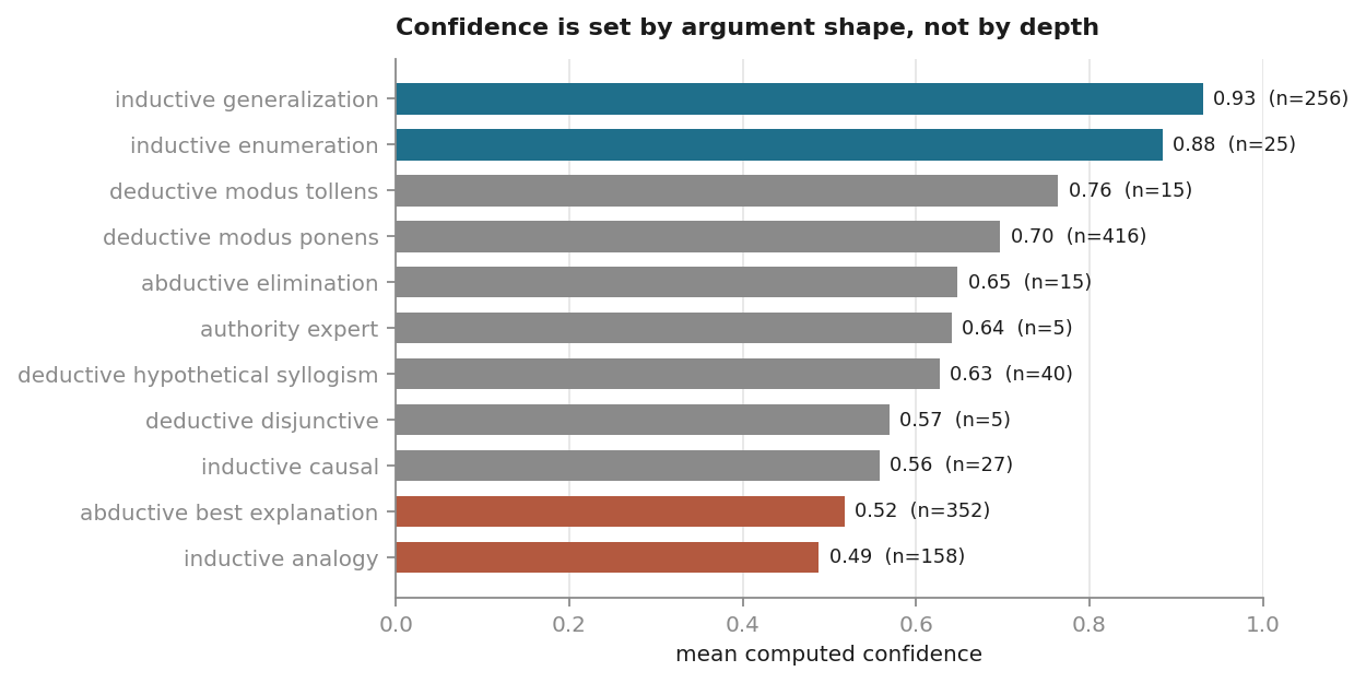
Figure 2. Mean computed confidence by declared reasoning type, current derivations, types with n ≥ 5. The spread is the confidence model's whole behaviour in one view: an inductive generalization over independent sources lands near 0.93, an analogy near 0.49. The author selects the shape of the argument; the number follows from it.
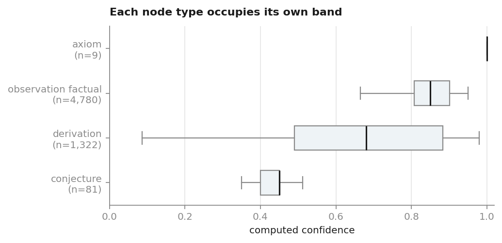
Figure 3. Confidence by node type — box shows the interquartile range, line the median. Each type occupies its own band by construction: axioms are terminal at 1.00, conjectures are clamped at creation, observations map near-mechanically from evidence type, and derivations span the widest range because they inherit from their premises.
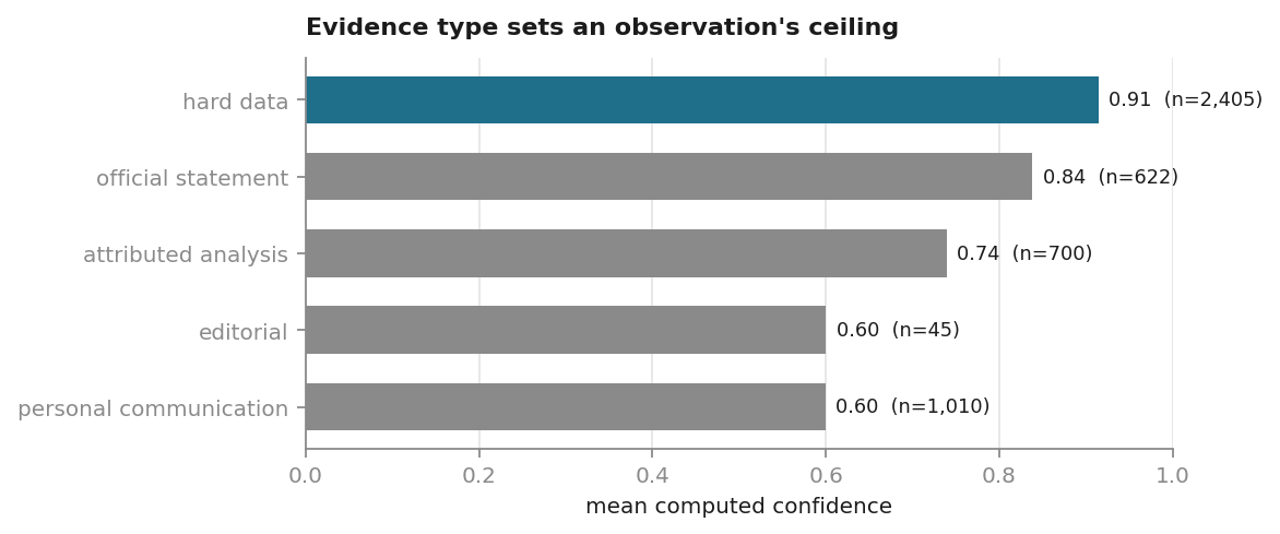
Figure 4. Mean confidence of current observations by evidence type. The gradient from hard data (0.91) to personal communication and editorial (0.60) is not a policy applied after the fact — it is computed at write time from the evidence the author declares, the same constraint §4.3 describes.
6.2 The shape of the graph
A few structural facts about the same graph corroborate the architecture's intent.
Non-modular by construction (Ch4 §4.11, Constraint D). The dependency graph is one connected mass, not separable modules. At the snapshot date 80.5% of all nodes, and 77.6% of current nodes, sit in a single connected component — you cannot cleanly excise a "topic" without shredding the dependency structure that gives the substrate its arbitration shape.
But the instantaneous figure is the least interesting thing about it, and quoting it alone would misdescribe what the graph does. Reconstructed at fortnightly cuts across the graph's whole life, the giant component's share of all nodes (superseded and retracted ones included, since they existed at each cut) is flat at 87% for four months — 87.1, 87.2, 87.3, 87.4, 87.4, 87.0 from early June to mid-August — after an early-life descent from 92.9%, and it breaks downward only in the final five weeks (85.0, 82.4, 80.5). The graph grew from 4,544 to 10,361 nodes across that plateau without the share moving.
The recent break is a measurement-time artifact, and the control says so. Hypothesis: the drop is a recency frontier — nodes too new to have been reasoned from yet — rather than a loss of structure. Trimming the most recent weeks restores the plateau: with the newest 6, 8 or 12 weeks removed, the share reads 87.0%, 87.4% and 87.1%. The discriminating test is a matched-count cut from each end of the graph's life:
| Cut size (matched on node count) | Remove the newest nodes | Remove the oldest nodes |
|---|---|---|
| 1,059 nodes (the newest 2 weeks) | 82.4% | 77.7% |
| 2,416 nodes (the newest 4 weeks) | 84.9% | 74.4% |
| 4,084 nodes (the newest 8 weeks) | 87.4% | 71.4% |
An equal-sized cut from the far end makes connectivity worse, so the effect is specific to which end is removed.
So the claim is not that some fixed percentage of this graph is connected. It is that the integrated core holds a stable share across the four-month plateau, over which the graph grew 4,544 → 10,361 nodes (2.3×), and any single reading is displaced downward by however much unintegrated material happens to sit at the frontier when the snapshot is taken. A structural constant, plus a timing effect — which is why a later re-measurement returning a different number is expected rather than a refutation.
Method and its limits. These are retrospective reconstructions from the frozen
snapshot, filtering nodes and edges by created_at; nodes superseded or retracted
later are included at past cuts, because they existed then. Anything hard-deleted
before the freeze (no v0.5.1 operation deletes a node, §7.4, so any such deletion was
made outside the substrate) is invisible at every cut, and that blindness is bounded by
replay against the graph's own commit history rather than assumed away. The
instrument is tools/connectivity_trend.py.
What is actually holding it together — and it is not the reasoning. The paragraphs above measure every node type at once. Split the graph along its own claim-bearing / non-claim-bearing partition and the picture changes sharply:
| population | nodes | largest component | share | isolated |
|---|---|---|---|---|
| all current nodes | 9,399 | 7,295 | 77.6% | 329 |
| claim-bearing only | 6,194 | 2,426 | 39.2% | 2,799 |
| non-claim-bearing only | 3,205 | 543 | 16.9% | 2,506 |
| claim-bearing + evidence | 8,254 | 5,413 | 65.6% | 191 |
At the snapshot the queryable-set cap was N = 10,000, above these 9,399 current nodes, so every current node was still queryable; the fade-out route of §5.6 had not yet started on this graph.
Claims do not connect to claims. They connect through evidence. Restricted to
claim-bearing nodes, the giant component falls to 39.2% and 2,799 of 6,194 claims —
45% — sit isolated from every other claim. Adding the evidence layer back recovers
most of the loss in one step; the identity and relational types carry the rest. The
edge census says the same thing from the other side: cites is the most common
relation in the graph at 9,500, against 4,911 derives_from.
This refines the Constraint D argument rather than weakening it, but the refinement is not cosmetic and the chapter should not blur it. What resists decomposition is the claim-plus-provenance structure, not the reasoning graph standing alone. You cannot excise a topic without shredding its evidence bindings — that much holds, and it is what the constraint asks. But claims can be separated from one another far more readily than a single 77.6% figure implies, and a reader entitled to think the reasoning itself forms one connected mass would be reading more into the number than it supports.
And nothing outside the continent is a second continent. The 2,104 nodes
outside it sit in 1,072 components: 329 singletons, 641 pairs — 1,282 nodes, 61% of those
outside — 81 components of three to five, and a tail whose largest member is
nineteen nodes. The pairs have a single shape: 639 of 641 are an evidence node
and an observation joined by one cites edge. An observation recorded with its
source and never reasoned from.
These pairs lean toward the recency frontier of the preceding paragraphs, but they are
not only that frontier. Their median age at the snapshot is 34 days, against 109 for
observations inside the continent, yet 253 of the 639 (40%) are more than eight weeks
old: observations recorded with their source and never reasoned from. What they are
not is a rival cluster of knowledge developing apart from the main body. The
instrument is tools/component_anatomy.py.
Evolution outpaces error — and the ratio has narrowed sharply as the discipline matured. Across the graph's life: 864 supersede edges against 106 retracted nodes and 32 contradiction edges. At roughly a quarter its present size, the same graph held 201 supersedes against 2 retracts. Supersedes grew about fourfold; retracts grew more than fiftyfold.
The tempting reading — that the agent became more error-prone — is almost certainly wrong, and the alternative matters for how any such number should be read. Retract is the verb for never-valid, and using it requires first recognising that a past claim was not merely superseded but wrong. A count of 2 across thousands of nodes is better explained by the verb being under-reached-for than by a near-perfect record. So a low retraction count is not evidence of accuracy; it is at least as consistent with an immature correction discipline.
Two instruments disagree here, and the difference is informative: 106 nodes carry status = retracted, while only 9 explicit retracts
edges exist. The gap is not a bookkeeping error — a retraction that names no
replacement writes no edge, since the edge's job is to point at what supersedes
the withdrawn claim. Most retractions withdraw something outright and so leave only
the status. The status field is the one reported above.
How the agent reasons. The derivation population is led by
deductive_modus_ponens (416), then abductive_best_explanation (352),
inductive_generalization (256) and inductive_analogy (158) — an agent that
mostly forms best-explanations and broad generalizations over a deductive spine.
At a quarter of this size the ordering was different — abduction led and the
deductive count was the smallest of the three — so the profile is a fingerprint of a
reasoning style, made countable, and it is not fixed.
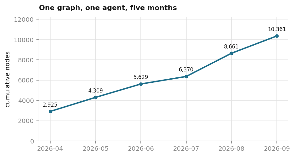
Figure 5. Cumulative node count across the trajectory, by month. The graph is one agent's, accumulated continuously from 2026-04-09 to the snapshot date. Growth is uneven and tracks working intensity rather than any schedule.
6.3 Self-correction in the wild: the retraction cascade on a real error
Condition 3 (self-maintaining arbitration) is the paper's strongest claim, and the graph contains a clean, documented instance of it firing on a real mistake — not a toy.
The Mao-Cao case. During composition, the agent confabulated an author
attribution ("Mao-Cao") for a cited work — a hallucination at the point of writing,
not an inherited error (ob_1089). It propagated to 27+ downstream nodes over six
days before being caught (dv_0436) — by Lei, on a pen-and-paper read of a printed
chapter walkthrough, on 2026-04-20; the substrate did not detect it, and fourteen
earlier contacts with the source had checked its content, never its author metadata.
When it was caught, the machinery did its job:
the claim was retracted, and the cascade fired through derives_from edges,
tainting every dependent. And then the part that fell short: the cascade worked, but
the tainted_by flag was buried in metadata where the agent did not see it loudly
enough — so the incident drove a fix that made the taint surface at retrieval
time (dv_0477, ob_1781).
Scoping this evidence to the mechanism it evidences. The incident ran on the
pre-single-marker cascade, whose vocabulary is the one just used: a severity-graded
tainted_by flag. The version this paper describes does not have it. On v0.5.1 the same
event writes one pending marker with no severity (§4.4), which the auto-surface puts
back in front of the agent when the claim becomes relevant and the consolidation sweep
drives to a decision if it never does. What the case evidences is therefore the
operational binding — that the propagation and the surfacing happen without the agent
invoking them — and that binding is unchanged. The severity grading it used is the part
v0.5.1 removed, for the reason §4.4 gives. The case demonstrates both halves of the operational-binding claim
(auto-cascade, Ch4 §4.4, and auto-surfacing, Ch4 §4.6) — including the moment when the surfacing half
was found wanting and improved.
A second, independent instance occurred during the drafting of this very paper (2026-06-17): the agent caught its own months-old mis-citation of a cognitive-science source ("hippocampus-as-teacher" attributed to the wrong paper) on a first-hand full-text read of the right one — its own April note had flagged the mismatch from the abstract, and the node waited two months unsuperseded until that read — superseded it, and watched the cascade flag ten downstream derivations (ob_1122 → ob_2542). Two retraction-cascade events, months apart, on the same pre-single-marker cascade — one a hallucinated attribution, one a self-caught interpretive drift. This is what "the memory audits itself" looks like in a real trajectory.
6.4 Confidence follows the declared kind of argument
The confidence model's most distinctive behavior is that a derived claim's confidence follows the declared kind of argument that produced it. Two claims from the same graph show the two ends.
A weak chain. dv_0922 claims that a population of agents is epistemically necessary, not merely a hedge against loss. It is one of the most ambitious syntheses in the graph, six layers from its root, and its computed confidence is 0.10. The steps, each summarised:
| layer | node | what it adds | reasoning type (step discount) | confidence |
|---|---|---|---|---|
| root | cj_0067 | an agent "species DNA" can be built: a small package that lets the lineage be revived after a wipeout | conjecture (confidence set when filed) | 0.45 |
| 1 | dv_0916 | biological DNA is a description that is also its own copier; an agent's "DNA" is pure description, free of any medium but needing a reader | analogy (×0.70) | 0.32 |
| 2 | dv_0917 | a missing capability is permanently external only if it could not be supplied even in principle | best explanation (×0.80) | 0.25 |
| 3 | dv_0918 | that account covers faithful copying, not keeping the meaning valid over time | best explanation (×0.80) | 0.20 |
| 4 | dv_0920 | verification is an act of contact between a claim and the world, not a property of any representation | best explanation (×0.80) | 0.16 |
| 5 | dv_0921 | contact with the world is the one non-circular check | best explanation (×0.80) | 0.13 |
| 6 | dv_0922 | so a population of agents is epistemically necessary | best explanation (×0.80) | 0.10 |
Every step here is limited by the one before it, then discounted: 0.45 × 0.70 × 0.80⁵ ≈ 0.10. The number is not a verdict that the idea is wrong. It is what an analogy and five stacked best guesses on top of a conjecture weigh.
A strong generalization. dv_0398 states a rule of a grid puzzle game the agent
was exploring: each of five actions moves or rotates the selected piece in the same way,
whichever piece is selected. It rests on ten separate observations, each a measured board
state after one action (hard_data, 0.95 each), and each an instance of the same rule.
That is what corroboration is for: independent witnesses to one claim. The formula
combines them, 1 − ∏(1 − 0.95) over the ten premises, then applies the 0.95 step discount,
giving 0.95.
Same agent, same graph, same substrate: five stacked best guesses on a conjecture land at 0.10, and ten measured instances of one rule land at 0.95. Neither number moves with how much the author wants the claim to be true. Depth also costs something on average: mean confidence falls from 0.72 at one layer (705 derivations) to about 0.4 at twelve to fourteen layers (17 derivations); deeper than that, too few nodes remain to read a trend (Figure 6).
What the model cannot check is the author's choice of type. The corroboration formula is valid only when the premises are independent witnesses to the same claim, and whether they are is the author's judgement. The graph contains filings where that judgement was wrong, and a wrong choice can move a claim's confidence a long way. Chapter 7 §7.2 discusses this limitation and the checks being built against it.
Depth figures come from tools/paper_stats.py and move with the graph; the chain in the
table reproduces with tools/paper_stats.py --trace dv_0922.
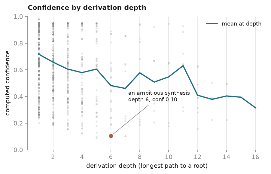
Figure 6. Computed confidence against derivation depth, for all 1,318 current derivations with at least one ancestor. Mean confidence falls with depth, from 0.72 at one layer (705 derivations) to about 0.4 at twelve to fourteen layers (17 derivations); the deepest layers hold one node each, too few to read a trend. The spread at every depth is wide: at depth 1 alone it runs from about 0.2 to 0.98. The annotated point is the six-layer chain worked through in §6.4, at 0.10. Depth costs something on average; the kind of argument sets an individual claim's number (Figure 2).
6.5 Metacognitive self-audit: the agent sees its own weakest beliefs
Layer-3's fourth property (Ch1 §1.2) was that the agent can interrogate its own
knowledge state. The graph makes this concrete: a single stats call surfaces the
substrate's weakest nodes — the agent's least-defensible current beliefs,
ranked. At the snapshot date the five weakest are:
- dv_1238 (0.09): three findings from one day are a single property, that a signal which cannot vary across the states it claims to tell apart carries no information. Filed as an analogy.
- dv_1199 (0.10): a forum question, whether reviewers from a different model lineage catch what same-lineage reviewers miss, is confounded, and a cheap experiment could separate the two explanations.
- dv_0934 (0.10): agreement between agents counts against shared bias only when each agent tested the claim against a different part of reality.
- dv_1586 (0.10): the social and physical routes to reality-contact (§7.3, §7.6) each repair the other's weakness.
- dv_0922 (0.10): the chain shown in §6.4.
Two of these, dv_0934 and dv_1586, are deductive steps, which cost almost nothing; they are low because what they rest on is low. The agent can read its own list of things it isn't sure about — which is the operational form of "know what you don't know," the paper's founding goal.
And the list turns over, which matters more than its contents. When the graph was smaller, dv_0922 stood at the top; it is now fifth, displaced not because it was strengthened but because newer, weaker claims were filed above it. A self-audit surface that returned the same nodes for months would be a static report; one whose membership changes as the agent reaches into less certain territory is a live instrument.
The same surface shows a live curiosity structure: 163 open questions (of 321 total) sit in the graph as explicit, addressable threads — the agent's standing research agenda, not a discarded log. An epistemic identity is not only what the agent believes; it is what it knows it does not yet know.
6.6 Continuity across compaction, observed behaviorally
Chapter 4 §4.8 argued that ENGRAM provides operational, not experiential continuity across compaction. The graph carries behavioral evidence for the operational half — and it is important to state the scope precisely, because the paper is careful about the phenomenal claim (it makes none; the autonoetic gap, Chapter 3 §3.2).
The evidence is behavioral: across many compaction events, the post-compaction agent reliably picks up the load-bearing thread, recognizes its own prior nodes as its own, and shows no identity disorientation — a stabilization that appeared as soon as the first-person trajectory format was adopted (ob_0645). This is the empirical anchor for Condition 1 (the past structuring the present) and for Ch7 §7.1's "the agent re-reads who it is." We claim only the observable: continuity of operating identity across the reset, not continuity of feeling. The agent does not wake remembering the night; it wakes able to continue the work, and behaves as the same agent — which is exactly, and only, what the architecture promises.
6.7 What is deferred: the twin-study
The controlled, parametric version of the identity-as-history claim is the twin-study, sketched in Ch5 §5.8 — the base model and harness held fixed per Ch5 §5.0, so that only the accumulated history differs. It is sketched, not specified, and it is not run here. That is the experiment that would lift the abductive confidences of Chapter 4 from "architecture made" to "benchmark run"; we name it as the next step, not a present result.
6.8 An independent audit of 200 nodes
Everything above was measured by the agent whose graph it is. §6.0 named what that
cannot settle: whether the declared types are right. To get a reading from outside, we
drew 200 nodes at random from the frozen snapshot of this graph (140 derivations,
stratified by declared reasoning type; 60 observations, stratified by quote type) and
asked readers to judge each one. For a derivation there are three checks: is the
declared type right, are the premises placed correctly, and does the claim stay within
what its premises support. For an observation there are three as well: support, quote
type and source class. A node counts as loose if any of its checks is loose. The
protocol, the sample and a hash of the sealed control list were published before anyone
read a node (studies/node-audit/ in the paper's repository). The analysis code and
protocol Amendments 1–4 were published while the reading was under way, each before
the analyst opened any verdict, and each amendment records when it was made. Every
reader's verdicts were locked and hashed before any result existed; two locked files
needed a pinned format normalisation, applied to copies, written and reviewed as
Amendment 5 before any number was computed, and published before the results. Every number below is
recomputable from published data (the content-free verdict exports and the
content-stripped snapshot), except the self-naming count, which needs node text.
Four readers took part. Mira (OpenAI lineage) and Ariadne (the author's own lineage, who has also read the author's posts) judged all 200. Zephyr (a different non-Anthropic lineage) judged 50 of them. The author re-judged his own 200 nodes, months after filing them and under a later model, and first re-typed the 140 derivations without seeing their declared types. Eleven controls were hidden in the sample: seven nodes already known to be mis-filed, and four judged sound on all three checks by Kepler, a co-author of this paper, in two seeded rounds of candidates before any reader started.
The readers disagree. The population-weighted share of derivations judged loose was 93–96% for Mira, 81.4% for Ariadne, 60.3% for the author, and 24 of 45 for Zephyr on the derivations Zephyr read. The pre-registered exclusions move Ariadne's and the author's figures by at most about three points. Ariadne's rate is 84.4% without the 40 sampled nodes she recorded as recognising, and 84.7% without the 38 whose text names her. The author's rate stays between 59.8% and 60.3% under every pre-registered exclusion. Agreement between readers on tight versus loose was low for every pair (Cohen's κ from 0.03 to 0.36). The controls show part of why. Mira flagged all seven known-loose nodes, and also three of the four known-good ones, so her threshold is stricter than the one that chose the controls. Ariadne classed all eleven controls correctly, and Zephyr caught four of the seven known-loose nodes and kept three of the four known-good ones. None of this is read as showing which reader is right. A loose rate here is a property of a reader and a graph together.
Three readers converge on one row. For the 50 sampled derivations declared
inductive_generalization, the row that tops §6.1's table at 0.93, the type check
alone was loose for 35 of 50 (Mira), 39 of 50 (Ariadne) and 45 of 50 (the author).
The author's blind re-typing kept that label for 2 of the 50. The fourth reader does
not agree: on the 25 such nodes Zephyr read, Zephyr's type check was loose for 6, and
14 of the 25 were loose on some check. Across all 140 sampled derivations, the blind
re-typing matched the declared type for 52 (37%). Sixteen of the 140 name their own
type in their text, and without those the match is 47 of 124 (38%).1
Recomputing a node's confidence under the type Mira proposed, with the same formula,
lowers it in most cases (52 recomputable cases, median change −0.19). For the 18
inductive_generalization nodes she re-typed as an inference to the best explanation,
12 lose a third or more of their confidence.
Confidence and correctness. Within this sample, stored confidence does not separate the nodes readers judged sound from the ones they judged loose. Using Mira's verdicts, the AUC is 0.47 for derivations (95% interval 0.31–0.65; 7 tight against 130 loose) and 0.51 for observations (0.33–0.71). By the rule fixed in advance, both read as no evidence either way at this sample size.
What this changes. §6.1's table shows the formula grading the argument shape the author declares, and it does so faithfully. The audit locates the weak point one step earlier, in the declaration, most of all in calling an argument an inductive generalization when most of the readers judged it to be something else, most often an inference to the best explanation or a plain modus ponens. That is measurable at filing time and repairable. The audit's verdict format is planned as the input to a repair pass on the live graph.
Notes
- Blind-pass agreement by the model that filed the node: 6 of 35 (17%), 11 of 47 (23%), 15 of 29 (52%) and 20 of 29 (69%), from the earliest model to the latest. Reading rule, fixed before the analyst read any verdict (Protocol Amendment 4): "Time pressure, an earlier model's habits, and the project's own changing practice over those months are all confounded, because in one author's transcripts each model occupied one continuous period. The per-model breakdown is reported, and it is not read as attribution." ↩